F-rep and voxels

Introduction

The traditional technology for exact modeling in the computer-aided design (CAD) field is boundary representation (B-rep). This industrially proven technique gives an efficient way of handling geometric shapes with non-compromised accuracy. In many engineering applications, however, it is not necessary to maintain the explicit equations of the surface boundaries. Therefore other approaches can be employed to represent a shape. One of the alternative approaches is functional representation (F-rep) or functional modeling.

In this article, we overview the basics of functional modeling and describe the data framework serving as an alternative to the traditional B-rep. The employed data framework is named DDF (Discrete Distance Field). One can find the theoretical foundation of this approach with the corresponding bibliography in the seminal paper [Frisken et al, 2000].

The fundamental question of geometric modeling is whether a random point selected in the ambient (modeling) space belongs to a solid body or not. A software system capable of answering this (and many more) questions is called a geometric modeling kernel. The geometric kernels use different representation schemes [Requicha, 1980], such as constructive solid geometry, implicit, boundary representation, voxels, etc. Here we describe a relatively fresh look at modeling, which is a part of the emerging field-driven design paradigm. This approach employs two representation schemes: the functional shape representation, and the space decomposition (voxels).

The field-driven design extends the idea of implicit modeling. The latter assumes that a shape corresponds to an implicit scalar function $f(x)=0$, where $x \in R^3$ (this formalism can be generalized though). The function $f$ (that might be called a "potential function") allows evaluation at any point in the ambient space, thus defining a continuous scalar field.

Before going into the details of the field-driven design, it is worth comparing this approach with the widely used boundary representation. It appears that only two general modeling principles embrace different representation schemes. These principles are the Eulerian and Lagrangian approaches to modeling [0FPS blog].

Eulerian definition

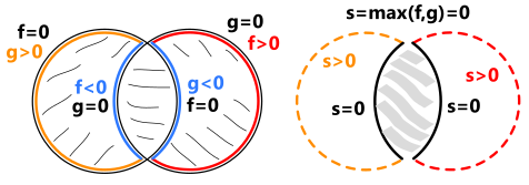
An implicit shape representation is a type of Eulerian representation which describes the modeled shape in terms of space it is embedded to. Formally, we define a map $f(x) = s$ where $f$ is a scalar function, and $s \in S$.

The shape being designed is then defined as the inverse map $f^{-1}$. For example, having $S_0=[-\infty,0] \subset S$, we can formalize shape $X$ as follows:

In functional modeling, the choice of $f$ and $S_0$ is somewhat arbitrary. The idea of this approach is to define the shape as a field in the ambient space. Selecting $f$ as a distance function induces the distance field in the ambient space. Similarly, one can define an "index field" for a set of solid bodies $B_0, B_1, ... ,B_N$ to attribute each point in the space with the object it belongs to: $f_i = i, x \in B_i$ and $f_i = 0$, otherwise.

The function $f$ does not have to be expressed with an analytic equation and can be defined procedurally, e.g., with a point-membership-classification (PMC) test. We will build upon this consideration later on, when expressing the potential function $f$ using voxelization of the ambient space.

Lagrangian definition

The Eulerian approach is contrasted to the Lagrangian representations such as precise B-rep or meshes. Instead of representing a shape as a map from the ambient space to some set of labels, a map from a parametric space to the ambient space is used.

One significant advantage of the Lagrangian shape definition is the straightforward way of sampling the boundary $\partial X$ (one has to traverse the parameter space, which usually has lower dimensionality than the ambient space). At the same time, solving the PMC problem is more complicated compared to the implicit schemes and generally requires the use of iterative methods. Another advantage of the Lagrangian definition is its compactness. While the implicit modeling technique seeks to describe the continuous space, the Lagrangian approach describes not space but an object embedded into the space.

Discrete distance fields

Overview

A fundamental graphical data structure that allows for representing the scalar fields in the ambient space is an octree. An octree serves as a carrier for the continuous scalar field whose values are associated with the vertices of the corresponding voxels. Introducing hierarchy allows models to take advantage of spatial locality: filled regions are clustered near each other, not randomly spread out in space.

The regularly sampled distance fields are computationally inefficient because of their significant size and consequently limited resolution. In contrast, the adaptively sampled distance fields (ADFs) allow for a detail-wise sampling with higher sampling rates in the curved areas and less dense sampling where the field varies smoothly.

In general, DDF is a tuple

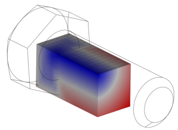
Here $f$ is the distance function (signed or unsigned), $H$ is a spatial hierarchy (e.g., octree), and $r$ is an optional reconstruction operator that allows converting the level set $f(x)=s$ to Lagrangian form. The most popular way of isosurface reconstruction is the Marching Cubes algorithm [Bourke, 1994] (see also the relevant overview and its following discussion at [0FPS blog]). If the gradient of the potential function is known, a manifold mesh representation can be generated with the more advanced Dual Contouring algorithm [Ju et al, 2002]. The following image illustrates an adaptively sampled distance function whose values are stored as the signed scalar values at voxel grid. Do you see a geometry of a bolt in there?

Voxel indexation in C++

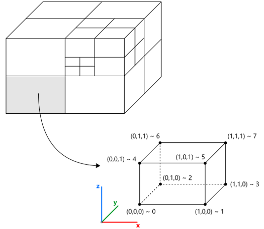
The voxelization is stored in the data structure named SVO (Sparse Voxel Octree), which is a hierarchy of parallelepiped cells. Each corner of a cell is numbered according to the following rule (C++ notations for bitwise shifts are used):

ID = nx | (ny << 1) | (nz << 2)

Here nx, ny, nz variables get the values of 0 and 1 depending on whether they represent min or max coordinate (the 3-tuple of these numbers is called a "corner location"). There is also a scalar value representing the distance to the shape from the corresponding cell vertex. The explicit coordinates of the corner points are not required, though they can be stored for convenience or maintenance needs. In Analysis Situs, we store them to be able to easily dump to VTU (VTK unstructured) format. The following picture gives a schematic view of an octree and the corner indexation in a cell.

The construction of the octree starts from the root node, which corresponds to the axis-aligned bounding box (AABB) of the object. The eight vertices of the root cells are supplemented with the distance values evaluated through the abstract interface of implicit function $f$. Depending on the distance field’s behavior in these eight vertices, a cell can be recursively split to octants. The following picture is the illustration of the splitting process. The numbering of octants follows the same rule as the numbering of vertices within one cell.

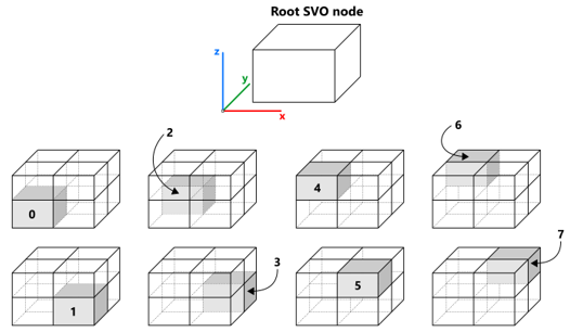
To switch back from the cell ID (in range [0,7]) to the corner location tuple, the following rule is used:

nx = (ID >> 0) & 1,
ny = (ID >> 1) & 1,
nz = (ID >> 2) & 1.

This rule gives the following correspondence:

ID | nx | ny | nz
 0 |  0 |  0 |  0
 1 |  1 |  0 |  0
 2 |  0 |  1 |  0
 3 |  1 |  1 |  0
 4 |  0 |  0 |  1
 5 |  1 |  0 |  1
 6 |  0 |  1 |  1
 7 |  1 |  1 |  1

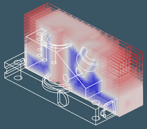
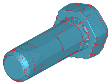
An SVO sub-hierarchy can be found in the octree by specifying its address as a sequence of cell IDs. The following picture illustrates SVO sub-hierarchy with IDs 0 $\to$ 0 for the bolt model. The inner space is shown in blue color. The outer space is shown in red color.

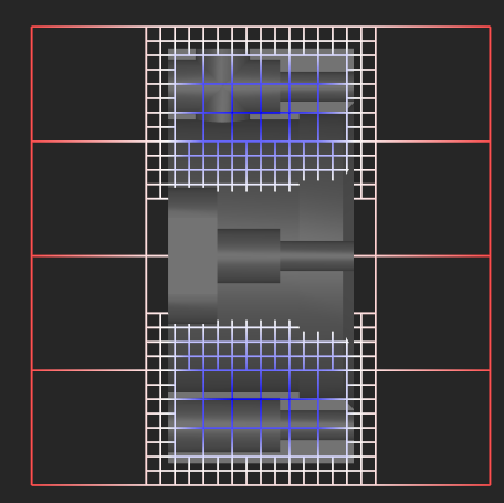
Instead of using bounding boxes, you might prefer using bounding cubes. The following picture illustrates a projection view of a clipped CNC model. You can notice that the model's inside get a less dense voxelization than its boundary.

Function evaluation

The key feature of the SVO data structure is its ability to evaluate the hosted potential function. I.e., the DDF voxelization behaves like a function itself.

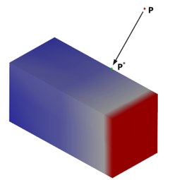
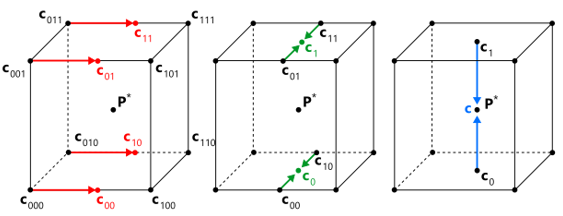
For the given point $\textbf{P} \in R^3$ and the voxel $V$, the evaluation of the field is done as follows. First, the point $\textbf{P}^*$ is derived by snapping the coordinates of the point $\textbf{P}$ to the voxel extents (if $\textbf{P} \in V$, then $\textbf{P}^* = \textbf{P}$). The following image illustrates snapping for a point $\textbf{P}$ resulted in the point $\textbf{P}^*$ nearest to the given input point.

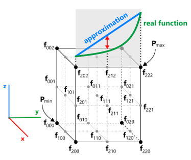
The point $\textbf{P}^*$ is classified w.r.t. the voxel $V$ and its octants recursively until the algorithm reaches the ultimate leaf $V^*$ containing $\textbf{P}^*$. The value of the potential function within the located voxel is computed by trilinear interpolation of the corner values as shown in the figure below.

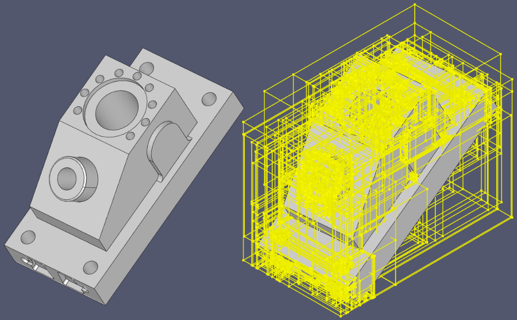
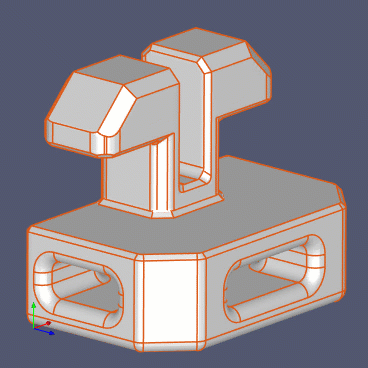
The distance values at the voxel’s corners are computed by projection of the corresponding points to the initial shape. The distance function being evaluated is represented with an abstract C++ class which allows for various implementations. For the sake of efficiency, the initial shape is tessellated and represented with a bounding volume hierarchy (BVH). The BVH allows for the fast intersection tests by quick filtering out the blocks that could not contain the result. The following image illustrates BVH for the sample ANC101 part.

Voxel splitting

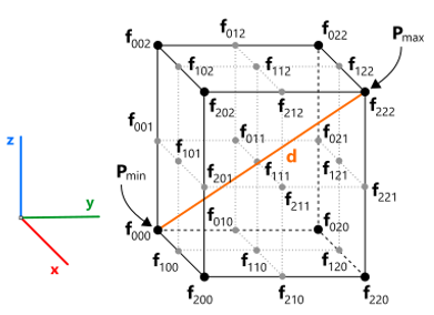
The voxelization process starts by constructing the root octree node initialized with the bounds of the distance function’s domain $D$. The domain $D$ is usually selected as the axis-aligned bounding box (or cube) of the shape being voxelized. The splitting procedure is based on function evaluation in 27 sample points corresponding to the corners of the current voxel and its potential splitting points. The following figure illustrates the sample points for testing the potential function on splitting. The $d$ value corresponds to the voxel's diagonal that can be used to control the grain size.

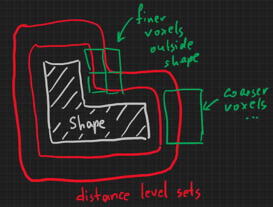
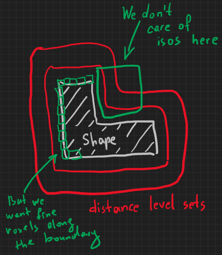
In DDF, the splitting process is driven by the idea to capture the distance field's features. This means that even empty space might get fine voxelization if the distance field varies significantly there (see the following sketch). Recall than DDF is the Eulerian representation, so its aim is to represent a spatial field, not just a boundary, that is nothing but a level set $f = 0$.

The precision of approximation is specified as the algorithm's input. Therefore, you can control the accuracy of the distance field approximation. Less accuracy means coarser voxelization.

Function domain

The domain of the potential function is a parallelepiped where the function $f$ is defined. Although the distance function is defined everywhere in the modeling space, it is more practical to have a notion of the domain to explicitly outline the volume which is considered as the object. Once this object volume (the domain) is defined, the distance field can be attached to the cells of this volume's decomposition structure $H$. To produce anisotropic voxels (cubes), the voxelization should start from a bigger box which will surround the initial domain located in the center of this box.

Polygonising scalar fields

It is worth mentioning that the functional modeling techniques per se do not require any polygonising, even for visualization (to render the F-rep model one can apply ray tracing techniques). Still, to communicate the modeling results to the downstream engineering applications, there is a need to convert the functional representation of a shape to something more conventional. Here we might want to switch from the Eulerian representation to Lagrangian one.

The most popular and simple algorithm for polygonising scalar fields is marching cubes dated at 1987 [Lorensen et al, 1987]. A review of some other techniques, including spatial decomposition, surface tracking, and shrink-wrapping can be found in [De Araujo et al, 2015].

The naive application of the marching cubes technique to an adaptive grid leads to the emergency of "cracks" (this effect is clearly explained in pp. 7-8 of [Shu et al, 1995]). Therefore, the marching cubes algorithm is usually applied to a regular grid obtained by discretization of the function's domain $D$. The finer discretization of the function domain yields a more precise reconstruction result. At the same time, since the initial data for the polygonising algorithm is the adaptive voxelization, it is highly desirable to produce the effectively decimated mesh. In the thesis [Keeter, 2013], the author uses the marching tetrahedrons algorithm that produces the adaptive triangulation that is not watertight. The author of this thesis argues that the non-watertight triangulation is enough for the rendering purposes. However, if the resulting mesh is intended for the further processing (e.g. numerical simulation or morphing), it is necessary to keep the mesh watertight and adaptive at the same time.

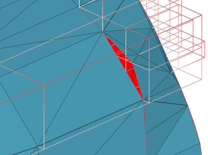
The following picture illustrates cracks (red color) in the mesh obtained by polygonising each cell of an adaptive octree independently.

And here is a closer look together with the voxelization cells:

As the alternative to the naive marching cubes approach, the adaptive dual contouring algorithm proposed by [Ju et al, 2002] can be considered (not available in Analysis Situs at the moment).

Derived point clouds

Principle

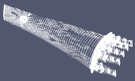
A point cloud with a feature-wise distribution of points can be naturally obtained from the adaptive voxelization. The density of a point cloud will be higher in the spatial zones where the input CAD model possesses its features. The easiest way to derive a point cloud is to sample each inner voxel in its center point. Take a voxelization of a turbine blade as an example:

And here is the derived point cloud:

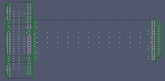
A point cloud derived by the naive sampling has insufficient accuracy near the boundary of a shape. Adding the voxels that intersect the boundary of the initial shape produces outliers as their center points unlikely belong to the surface. The following picture illustrates a DDF-derived point cloud composed of inner points (white) and quasi-boundary points (green).

Point cloud shape representation can be useful in machine learning applications as a compact shape descriptor.

Boundary projection

The points sampled in the boundary-crossing voxels do not lie on the boundary of the shape. To snap these points to the boundary, two techniques can be proposed:

1. Since the distance field is completely defined in a voxel, the corresponding piece of surface can be reconstructed locally in that voxel. Such a local polygonising can be achieved with the marching cubes method. Then, a point can be projected to the locally reconstructed piece of surface.
2. The points can be projected directly to the faceted representation of the initial shape. To speed up the projection routine, the bounding volume hierarchy structure (BVH) can be used.

Although the local polygonising looks like a natural completion to the entire method, it appears that the voxel-to-surface mapping suffers from the following deficiencies. First, the marching cubes algorithm may sometimes end up with non-manifold or even disconnected surfaces. Second, the polygonised surface $s_1$ is only an approximation to the original boundary $s_0,$ thus the membership classification of the projected point $\textbf{P}_i^*$ remains undefined (the PMC test may return different results for the two surfaces).

To avoid the undefined PMC status, the initial surface $s_0$ should be used for the global projection (as opposed to the local projection on marching cubes’ result). The fast global projection is done with the help of BVH decomposition of the initial shape. It should be noted that the BVH decomposition is already available at this stage of computation as it is used as a backbone of the distance function. Therefore, there is no extra overhead for the BVH construction.

Applications

The voxelization apparatus used in the field-based design can be adapted to cover different application needs, such as:

1. General-purpose modeling and Boolean operations. People tend to attribute the distance field approaches as much more reliable than traditional B-rep. However, we think that F-rep is still a boutique business.
2. Material removal simulation [Sullivan et al, 2012].
3. Mesh repair, including shrink wrapping techniques.
4. Constructing the derived part representations, such as adaptive point clouds, unstructured grids, etc. Such customizations concern the $r$ (reconstruction/polygonizing) operator of the DDF framework.
5. Filling parts with lattices [Pasko et al, 2011].

Computing Boolean operations on implicit surfaces corresponds to an appropriate application of min/max operations on the input distance fields. The authors of [Pavic et al, 2010] use the adaptive octrees to gain finer resolution in the spatial zones where the operands of a Boolean algorithm interfere. Therefore, the voxelization in this context is driven not by the distance function but by another property of the input (the customization of the DDF framework is related to the implicit function $f$).

Splitting strategies

Although this article is mainly devoted to DDF, we should not forget that some applications do not really require the adaptively sampled distance fields. Instead, you might want to have just an adaptive voxelization, which is not obliged to capture all the features of the spatially varying distance field. Although the underlying sparse voxel octree (SVO) data structure remains largely the same, there are several questions you might want to think about to get the most efficient yet practical voxelization approach.

1. Do you really need to capture some "potential function" (like distance) in the ambient space, or do you rather want to voxelize the existing Lagrangian shape representation?
2. Would you like to sacrifice some extra memory to store custom attributes in your voxels, such as pre-evaluated function values (the scalars)?
3. What would be the voxel splitting criterion? We have outlined one above, but it might be something completely custom.

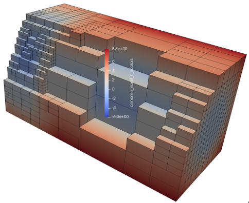
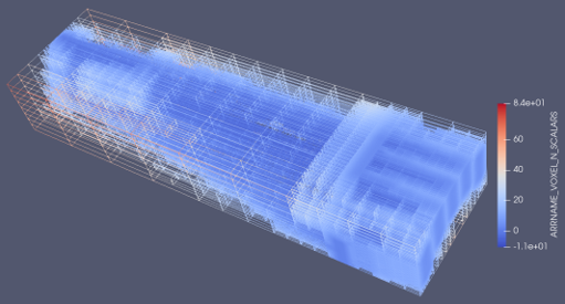
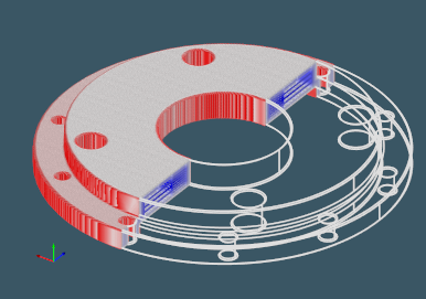
One broadly used voxelization strategy consists is splitting up those spatial cells that contain real geometry, while leaving the outer and inner voxels intact. This way, we do not try to approximate the varying isosurfaces of the implicit distance fields and just discretize the existing shape's boundary. If the voxelization is done not taking into account the distance field approximation criterion, it could lead to very dense decompositions, like the one shown in the following figure (more than 1 million voxels):

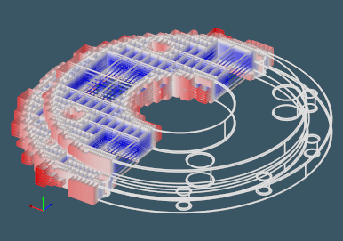
However, it might make little sense to decompose the planar regions where curvature is close to zero. This is where you might want to control the accuracy of the distance field approximation again (~35k voxels for the precision of 0.5 [mm]):

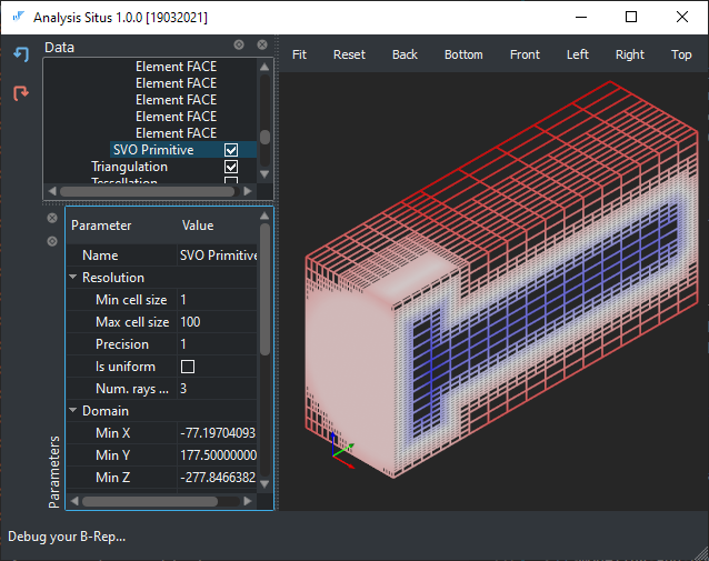
Use in Analysis Situs

To build voxelization for the given CAD or mesh geometry, use the following Tcl command of Analysis Situs:

This function creates a new octree Node in the project tree, where you can then configure different aspects of voxelization.