Thickness distribution
Overview
Two methods for thickness calculation are widely adopted in the CAD/CAM/CAE applications:
- Ray-based method.
- Sphere-based method.
The ray-based method measures the thickness value at each point by casting a ray orthogonally to that point until the intersection with the opposite surface element. The sphere-based method attempts to inscribe spheres in the solid body instead.
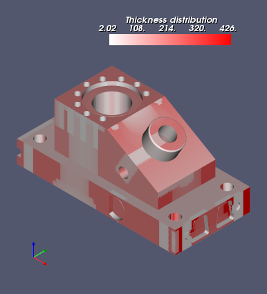
The following image illustrates the thickness map obtained with the ray-based method. You can see that inner features (such as holes) leave their imprints in the distribution when mapped to the color scale.
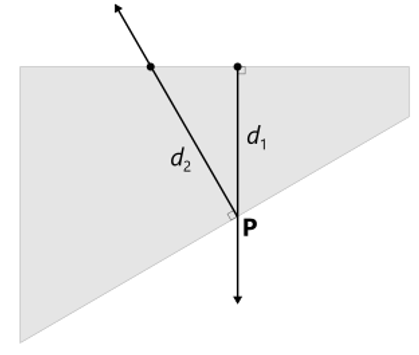
While the ray-based method is somewhat easier to implement, the thickness distribution obtained with that method is ambiguous. E.g., take a look at the point P in the figure below. While we can use a convention that the thickness value at this point is the value d2 measured by shooting a ray from this point, one could argue that the better value is d1 from the incoming ray. Therefore, there is inherent ambiguity attached to the ray-based method.
In contrast, the sphere-based method does not suffer from such an ambiguity. It yields the results that are consistent with the mechanical drawing definition of thickness. In the sphere-based method, the thickness value at a point P is defined as a diameter of the maximum inscribed sphere (MIS) contacting the surface at this point. The locus of the center points of the inscribed spheres constitutes the medial surface (medial axis in 2D) of a CAD model. The method described in [Inui et al, 2015] uses distance fields hosted at voxelization to calculate the diameters of the inscribed spheres.
In [Inui et al, 2016], the authors propose a method of shrinking spheres, which can be implemented using the same algorithmic core as in the ray-based method. Both approaches start from a triangulation covering the boundary of a CAD model. To obtain accurate results, the initial mesh should be fine enough. The shrinking spheres method attempts to construct a series of MIS starting from the mean point of each triangle. From each mean point, the algorithm casts a ray in the direction opposite to the surface normal. The midpoint between the ray source and its closest intersection is taken as the initial center of a sphere. All triangles intersected by this sphere are collected, and the closest one is chosen to shrink the initial guess. The shrinking procedure stops when the radius of the newly generated sphere is stabilized at some value, which is taken as the result. For the ray-triangle and triangle-sphere intersection tests, the algorithms from the monograph [Ericson, 2005] can be employed. In the broad-phase of the intersection, these algorithms use the bounding volume hierarchy structures (BVH) constructed on the axis-aligned bounding boxes (AABB) to which the initial CAD model is decomposed after the surface meshing.
Run thickness analysis
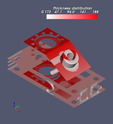
To run thickness computation, use check-thickness command. Once executed, you can select the newly created Thickness Node in the Object Browser and tune the algorithm's parameters. One option is to specify a fixed direction for the thickness measurement. The following figure illustrates thickness distribution map for OZ direction. The mesh elements having no associated thickness values (e.g., because they are parallel to the test ray) are not rendered.
The thickness map can be computed for mesh Nodes as well as for the primary Part Node. In the latter case, the visualization facets available in the corresponding B-rep structures will be used. Since the visualization facets are essentially sparse, using them is not recommended as it badly affects the accuracy of the thickness map.